Detecting Anomalies in Images Using Computer Vision–Based Regression Models
Anomaly detection is a critical task in various industries, including manufacturing, healthcare, security, autonomous systems, energy, utility, oil and gas. Traditional methods rely on explicit rules or statistical thresholds, which often struggle to handle complex visual data.
Using computer vision, along with deep learning and regression models, enables us to analyze patterns in images and identify deviations from the norm.
In this article, we delve into how we can apply regression models in anomaly detection, the workflow involved, the methodologies we can employ, and the industry best practices.
Understanding Anomaly Detection in Images
Anomalies in images mean the patterns or objects that deviate significantly from the norm. Real-world examples include defects in manufactured products, irregularities in medical scans, damages in gas or oil pipelines, and unusual activities in surveillance footage.
Unlike classification tasks, anomaly detection often lacks predefined labels for anomalies, requiring us to train models to learn the “normal” distribution and identify outliers.
Regression models are particularly useful in anomaly detection because they predict continuous values, such as pixel intensities or feature reconstructions. The difference between the predicted and actual values indicates the likelihood of an anomaly.
Key Technologies and Approaches for Anomaly Detection
We can employ several approaches that use computer vision techniques and regression models to detect anomalies:
Autoencoders
Autoencoders are neural networks we train to compress and reconstruct input images. The reconstruction error (difference between input and output) serves as an anomaly score. Anomalies typically have higher reconstruction errors since they deviate from the normal patterns the autoencoder learned.
Variational Autoencoders or VAEs: A probabilistic extension of autoencoders that models the latent space as a distribution, enhancing the ability to generalize normal patterns.
Convolutional Neural Networks or CNNs
CNNs allow us to extract high-level features from images, which we feed into regression models to predict pixel-level or patch-level intensities. These models can highlight regions where the prediction deviates significantly, signaling anomalies.
Generative Adversarial Networks or GANs
GANs consist of a generator and a discriminator. The generator learns to produce realistic images, while the discriminator differentiates between real and generated images. We detect anomalies using:
Reconstruction Error: Generated images deviate more for anomalies.
Discriminator Output: The discriminator’s confidence decreases for anomalous inputs.
Feature-Based Regression Models
By utilizing pre-trained CNNs like ResNet or EfficientNet, we extract image features and feed them into a regression model. The model predicts a target variable such as expected pixel values or an embedding representing the normal state. Deviations from predictions indicate anomalies.
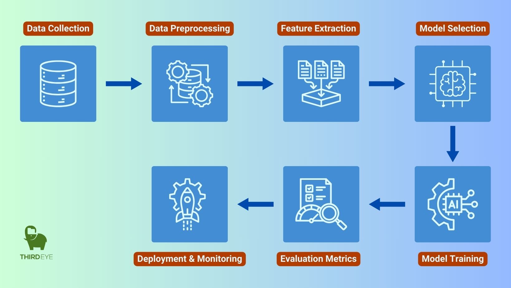
Workflow for Anomaly Detection Using Computer Vision-based Regression Model
The typical workflow for detecting anomalies using a computer vision-based regression model involves:

Data Collection and Preprocessing
Dataset Acquisition: Usually, we begin by collecting a dataset consisting primarily of normal images. If available, we can also include a small set of anomalies to assist in evaluation.
Data Cleaning: We remove noise and ensure that the dataset accurately represents normal patterns is essential.
Preprocessing: We use techniques such as normalization, resizing, and augmentation to ensure consistent input quality and help the model generalize.
Feature Extraction
Pre-trained Models: We can use pre-trained CNNs, such as ResNet or VGG, to extract meaningful features from images. These networks, trained on large volumes of datasets, provide us with a robust starting point.
Custom Feature Extractors: In cases where domain-specific features are necessary, we can design and train custom CNNs.
Here’s a sample of using a pre-trained model like ResNet for feature extraction:
from tensorflow.keras.applications import ResNet50
from tensorflow.keras.models import Model
# Load pre-trained ResNet50
resnet = ResNet50(weights=’imagenet’, include_top=False, input_shape=(128, 128, 3))
# Feature extractor model
feature_extractor = Model(inputs=resnet.input, outputs=resnet.layers[-2].output)
# Extract features from image batch
image_batch = np.random.rand(10, 128, 128, 3) # Example batch of images
features = feature_extractor.predict(image_batch)
print(features.shape) # Outputs: (10, Feature_Size)
Model Selection and Training
Choosing the Model: Depending on the complexity of the task, we can choose between autoencoders, GANs, or regression-based deep learning models.
Training: We can train the models using only normal data, with the objective of minimizing reconstruction or regression errors. This ensures the model learns the standard patterns effectively.
Validation: Cross-validation techniques can be employed to monitor the model’s performance and prevent overfitting.
For example, we are building and training an autoencoder for anomaly detection:
from tensorflow.keras.models import Model
from tensorflow.keras.layers import Input, Conv2D, MaxPooling2D, UpSampling2D
# Autoencoder Architecture
input_img = Input(shape=(128, 128, 1))
x = Conv2D(32, (3, 3), activation=’relu’, padding=’same’)(input_img)
x = MaxPooling2D((2, 2), padding=’same’)(x)
x = Conv2D(64, (3, 3), activation=’relu’, padding=’same’)(x)
encoded = MaxPooling2D((2, 2), padding=’same’)(x)
x = Conv2D(64, (3, 3), activation=’relu’, padding=’same’)(encoded)
x = UpSampling2D((2, 2))(x)
x = Conv2D(32, (3, 3), activation=’relu’, padding=’same’)(x)
x = UpSampling2D((2, 2))(x)
decoded = Conv2D(1, (3, 3), activation=’sigmoid’, padding=’same’)(x)
autoencoder = Model(input_img, decoded)
autoencoder.compile(optimizer=’adam’, loss=’mse’)
# Training the Autoencoder
autoencoder.fit(train_images, train_images,
epochs=50, batch_size=32,
validation_split=0.1)
Evaluation Metrics
Reconstruction Error: Calculating pixel-wise or feature-wise reconstruction errors provides an anomaly score.
Precision, Recall, and F1 Score: These metrics are applied when labeled anomaly data is available, provide us insights into detection accuracy.
ROC Curve: We use ROC curve to assess the model’s sensitivity and specificity by plotting the true positive rate against the false positive rate.
Here’s an example of using reconstruction error for anomaly detection:
# Calculate Reconstruction Error
reconstructed_images = autoencoder.predict(test_images)
reconstruction_error = np.mean((test_images – reconstructed_images) ** 2, axis=(1, 2, 3))
# Setting an anomaly threshold
threshold = np.percentile(reconstruction_error, 95)
# Classify anomalies
anomalies = reconstruction_error > threshold
print(“Number of anomalies detected:”, np.sum(anomalies))
Deployment and Monitoring
Integration: The trained model can be integrated into real-time systems or batch processing workflows.
Monitoring: Regular monitoring is important to ensure the model maintains performance as new data is encountered. Retraining with updated datasets is performed when necessary.
For example, we are deploying the model on edge devices with TensorFlow Lite:
import tensorflow as tf
# Convert Keras model to TensorFlow Lite
converter = tf.lite.TFLiteConverter.from_keras_model(autoencoder)
tflite_model = converter.convert()
# Save the model
with open(‘autoencoder_model.tflite’, ‘wb’) as f:
f.write(tflite_model)
# Load and run on an edge device
interpreter = tf.lite.Interpreter(model_path=’autoencoder_model.tflite’)
interpreter.allocate_tensors()
input_details = interpreter.get_input_details()
output_details = interpreter.get_output_details()
# Preparing input for inference
input_data = np.expand_dims(preprocess_image(“path/to/test_image.jpg”), axis=0).astype(np.float32)
interpreter.set_tensor(input_details[0][‘index’], input_data)
# Run inference
interpreter.invoke()
output_data = interpreter.get_tensor(output_details[0][‘index’])
print(“Inference result shape:”, output_data.shape)
This comprehensive workflow ensures that each step, from data collection to deployment, is meticulously handled to achieve reliable anomaly detection accuracy rate.
Case Studies and Applications
Computer Vision-based anomaly detection approaches are delivering tangible results across industries. Let’s explore some real-world case studies that highlight the efficacy and versatility of these approaches:
Industrial Quality Control
In manufacturing, the regression-based models detect surface defects in products such as metal sheets, plywood boards, or circuit boards. These models achieve over 90% accuracy in identifying scratches, dents, uneven density or misalignment.
Medical Imaging
We can analyze X-rays, MRIs, and CT scans using regression models to identify anomalies like tumors or fractures. By learning normal anatomy patterns, these models highlight areas of concern for further examination, assisting doctors in the treatment process.
Security and Surveillance
For anomaly detection in surveillance footage, we can identify unusual activities, such as unauthorized access or suspicious objects. Regression models focus on pixel-level changes to detect subtle anomalies.
Challenges and Suggested Solutions
Data Scarcity Challenge
Obtaining sufficient normal and anomalous samples can be challenging sometimes.
Solution: We can utilize data augmentation, synthetic data generation, or transfer learning to overcome data scarcity.
Complexity of Anomalies
Anomalies are often diverse and unpredictable.
Solution: Hybrid models combining deep learning with domain-specific heuristics or probabilistic frameworks address this challenge.
Computational Costs
Training deep models on large datasets requires significant resources.
Solution: We can use techniques like pruning, quantization, and knowledge distillation optimize models for edge computing.
Evaluation without Labels
Ground truth for anomalies may not be available sometimes.
Solution: We can use unsupervised evaluation metrics and active learning to iteratively refine model performance.
Future Directions
Looking ahead, we are committed to advancing the capabilities of anomaly detection with innovative strategies:
Self-Supervised Learning: Models that can learn representations without extensive labeled data.
Hybrid Approaches: Combining regression models with probabilistic frameworks for better generalization.
Edge Deployment: Optimizing models for real-time anomaly detection on edge devices.
Conclusion
By implementing regression-based approaches to anomaly detection, we can significantly enhance our ability to detect and address critical issues in real-time. This rapidly evolving field holds great promise for achieving more accurate, scalable, and efficient solutions across diverse applications.
References
- Bergmann, P., Fauser, M., Sattlegger, D., & Steger, C. (2019). “MVTec AD—A Comprehensive Real-World Dataset for Unsupervised Anomaly Detection.”
- Goodfellow, I., Pouget-Abadie, J., Mirza, M., et al. (2014). “Generative Adversarial Networks.”
- Kingma, D. P., & Welling, M. (2013). “Auto-Encoding Variational Bayes.”
- Zhou, Z., Siddiquee, M. M., Tajbakhsh, N., & Liang, J. (2018). “Unet++: A Nested U-Net Architecture for Medical Image Segmentation.”


