Example Dataset

For this example, we will use a sample of data from the Home Credit Default Risk machine learning competition on Kaggle. (To get started with the competition, see this article). The entire dataset is available for download and here we will use a sample for illustration purposes.

The competition is a supervised classification problem and this is a good dataset to use because it has many missing values, numerous highly correlated (collinear) features, and a number of irrelevant features that do not help a machine learning model.

Creating an Instance

To create an instance of the FeatureSelector class, we need to pass in a structured dataset with observations in the rows and features in the columns. We can use some of the methods with only features, but the importance-based methods also require training labels. Since we have a supervised classification task, we will use a set of features and a set of labels.

(Make sure to run this in the same directory as feature_selector.py )

from feature_selector import FeatureSelector

# Features are in train and labels are in train_labels
fs = FeatureSelector(data = train, labels = train_labels)

Methods

The feature selector has five methods for finding features to remove. We can access any of the identified features and remove them from the data manually, or use the remove function in the Feature Selector.

Here we will go through each of the identification methods and also show how all 5 can be run at once. The FeatureSelector additionally has several plotting capabilities because visually inspecting data is a crucial component of machine learning.

Missing Values

The first method for finding features to remove is straightforward: find features with a fraction of missing values above a specified threshold. The call below identifies features with more than 60% missing values (bold is output).

fs.identify_missing(missing_threshold = 0.6)

17 features with greater than 0.60 missing values.

We can see the fraction of missing values in every column in a dataframe:

fs.missing_stats.head()

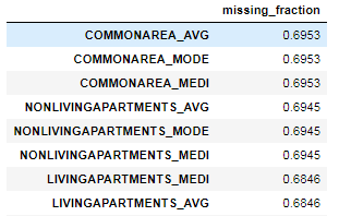
To see the features identified for removal, we access the ops attribute of the FeatureSelector , a Python dict with features as lists in the values.

missing_features = fs.ops['missing']
missing_features[:5]

['OWN_CAR_AGE',
 'YEARS_BUILD_AVG',
 'COMMONAREA_AVG',
 'FLOORSMIN_AVG',
 'LIVINGAPARTMENTS_AVG']

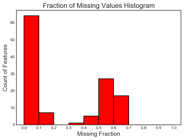
Finally, we have a plot of the distribution of missing values in all feature:

fs.plot_missing()

Collinear Features

Collinear features are features that are highly correlated with one another. In machine learning, these lead to decreased generalization performance on the test set due to high variance and less model interpretability.

The identify_collinear method finds collinear features based on a specified correlation coefficient value. For each pair of correlated features, it identifies one of the features for removal (since we only need to remove one):

fs.identify_collinear(correlation_threshold = 0.98)

21 features with a correlation magnitude greater than 0.98.

A neat visualization we can make with correlations is a heatmap. This shows all the features that have at least one correlation above the threshold:

fs.plot_collinear()

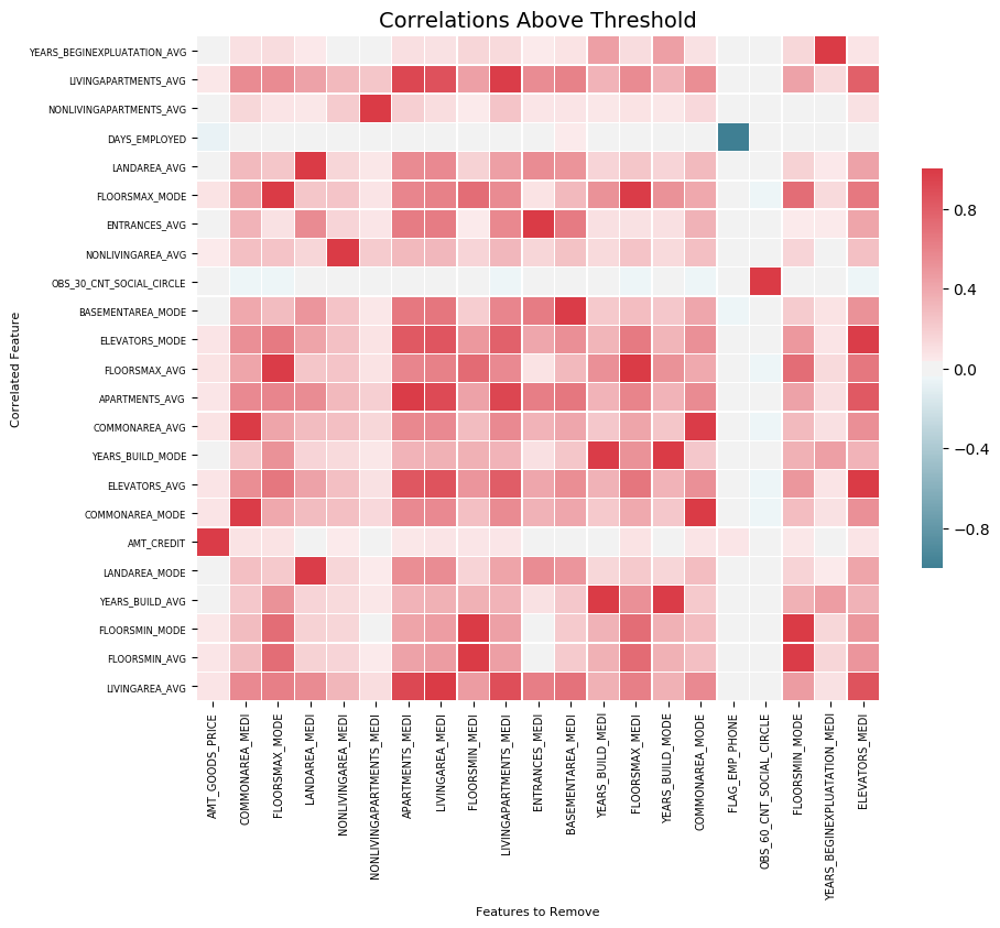
As before, we can access the entire list of correlated features that will be removed, or see the highly correlated pairs of features in a dataframe.

# list of collinear features to remove
collinear_features = fs.ops['collinear']

# dataframe of collinear features
fs.record_collinear.head()

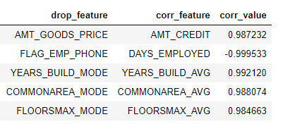
If we want to investigate our dataset, we can also make a plot of all the correlations in the data by passing in plot_all = True to the call:

Zero Importance Features

The previous two methods can be applied to any structured dataset and are deterministic — the results will be the same every time for a given threshold. The next method is designed only for supervised machine learning problems where we have labels for training a model and is non-deterministic. The identify_zero_importance function finds features that have zero importance according to a gradient boosting machine (GBM) learning model.

With tree-based machine learning models, such as a boosting ensemble, we can find feature importances. The absolute value of the importance is not as important as the relative values, which we can use to determine the most relevant features for a task. We can also use feature importances for feature selection by removing zero importance features. In a tree-based model, the features with zero importance are not used to split any nodes, and so we can remove them without affecting model performance.

The FeatureSelector finds feature importances using the gradient boosting machine from the LightGBM library. The feature importances are averaged over 10 training runs of the GBM in order to reduce variance. Also, the model is trained using early stopping with a validation set (there is an option to turn this off) to prevent overfitting to the training data.

The code below calls the method and extracts the zero importance features:

# Pass in the appropriate parameters
fs.identify_zero_importance(task = 'classification', 
                            eval_metric = 'auc', 
                            n_iterations = 10, 
                             early_stopping = True)

# list of zero importance features
zero_importance_features = fs.ops['zero_importance']

63 features with zero importance after one-hot encoding.

The parameters we pass in are as follows:

• task : either “classification” or “regression” corresponding to our problem
• eval_metric: metric to use for early stopping (not necessary if early stopping is disabled)
• n_iterations : number of training runs to average the feature importances over
• early_stopping: whether or not use early stopping for training the model

This time we get two plots with plot_feature_importances:

# plot the feature importances
fs.plot_feature_importances(threshold = 0.99, plot_n = 12)

124 features required for 0.99 of cumulative importance

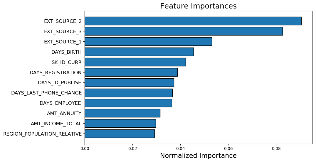
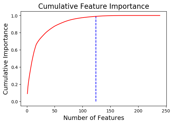
On the left we have the plot_n most important features (plotted in terms of normalized importance where the total sums to 1). On the right we have the cumulative importance versus the number of features. The vertical line is drawn at threshold of the cumulative importance, in this case 99%.

Two notes are good to remember for the importance-based methods:

• Training the gradient boosting machine is stochastic meaning the feature importances will change every time the model is run

This should not have a major impact (the most important features will not suddenly become the least) but it will change the ordering of some of the features. It also can affect the number of zero importance features identified. Don’t be surprised if the feature importances change every time!

• To train the machine learning model, the features are first one-hot encoded. This means some of the features identified as having 0 importance might be one-hot encoded features added during modeling.

When we get to the feature removal stage, there is an option to remove any added one-hot encoded features. However, if we are doing machine learning after feature selection, we will have to one-hot encode the features anyway!

Low Importance Features

The next method builds on zero importance function, using the feature importances from the model for further selection. The function identify_low_importance finds the lowest importance features that do not contribute to a specified total importance.

For example, the call below finds the least important features that are not required for achieving 99% of the total importance:

fs.identify_low_importance(cumulative_importance = 0.99)

123 features required for cumulative importance of 0.99 after one hot encoding.
116 features do not contribute to cumulative importance of 0.99.

Based on the plot of cumulative importance and this information, the gradient boosting machine considers many of the features to be irrelevant for learning. Again, the results of this method will change on each training run.

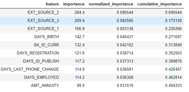
To view all the feature importances in a dataframe:

fs.feature_importances.head(10)

The low_importance method borrows from one of the methods of using Principal Components Analysis (PCA) where it is common to keep only the PC needed to retain a certain percentage of the variance (such as 95%). The percentage of total importance accounted for is based on the same idea.

The feature importance based methods are really only applicable if we are going to use a tree-based model for making predictions. Besides being stochastic, the importance-based methods are a black-box approach in that we don’t really know why the model considers the features to be irrelevant. If using these methods, run them several times to see how the results change, and perhaps create multiple datasets with different parameters to test!

Single Unique Value Features

The final method is fairly basic: find any columns that have a single unique value. A feature with only one unique value cannot be useful for machine learning because this feature has zero variance. For example, a tree-based model can never make a split on a feature with only one value (since there are no groups to divide the observations into).

There are no parameters here to select, unlike the other methods:

fs.identify_single_unique()

4 features with a single unique value.

We can plot a histogram of the number of unique values in each category:

fs.plot_unique()

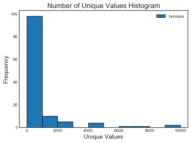
One point to remember is NaNsare dropped before calculating unique values in Pandas by default.

Removing Features

Once we’ve identified the features to discard, we have two options for removing them. All of the features to remove are stored in the opsdict of the FeatureSelector and we can use the lists to remove features manually. Another option is to use the remove built-in function.

For this method, we pass in the methods to use to remove features. If we want to use all the methods implemented, we just pass in methods = 'all'.

# Remove the features from all methods (returns a df)
train_removed = fs.remove(methods = 'all')

['missing', 'single_unique', 'collinear', 'zero_importance', 'low_importance'] methods have been run

Removed 140 features.

This method returns a dataframe with the features removed. To also remove the one-hot encoded features that are created during machine learning:

train_removed_all = fs.remove(methods = 'all', keep_one_hot=False)

Removed 187 features including one-hot features.

It might be a good idea to check the features that will be removed before going ahead with the operation! The original dataset is stored in the dataattribute of the FeatureSelector as a back-up!

Running all Methods at Once

Rather than using the methods individually, we can use all of them with identify_all. This takes a dictionary of the parameters for each method:

fs.identify_all(selection_params = {'missing_threshold': 0.6,    
                                    'correlation_threshold': 0.98, 
                                    'task': 'classification',    
                                    'eval_metric': 'auc', 
                                    'cumulative_importance': 0.99})

151 total features out of 255 identified for removal after one-hot encoding.

Notice that the number of total features will change because we re-ran the model. The remove function can then be called to discard these features.

Conclusions

The Feature Selector class implements several common operations for removing features before training a machine learning model. It offers functions for identifying features for removal as well as visualizations. Methods can be run individually or all at once for efficient workflows.

The missing,collinear, and single_unique methods are deterministic while the feature importance-based methods will change with each run. Feature selection, much like the field of machine learning, is largely empiricaland requires testing multiple combinations to find the optimal answer. It’s best practice to try several configurations in a pipeline, and the Feature Selector offers a way to rapidly evaluate parameters for feature selection.

As always, I welcome feedback and constructive criticism. I want to emphasis that I’m looking for help on the FeatureSelector. Anyone can contribute on GitHub and I appreciate advice from those who just uses the tool! I can also be reached on Twitter @koehrsen_will.