Recently I started working on a Python package which is everything time series, with specific focus on EDA, forecasting, classification and anomaly detection. It will leverage other Python libraries wherever appropriate. My first realization was that I need a Python module to generate synthetic time series data. This post is all about synthetic data generation for time series. Our generation example will be a time series with trend, seasonal cycle and random noise. It’s part of of new Python package zaman, which is in the work in progress stage right now. The source code is in the GitHub repo whakapai. The repo contains source for several data science Python packages.
What is Time Series Data
Various kinds of time series generation is supported. Currently it supports the following 9 types of time series. More will be added in future. For each of these types of time series the generation process is controlled with a set of configuration parameters.
- Random walk
- Trend, seasonal cycle and random noise
- Superposition of multiple sine function with random noise
- Exponential auto regressive with noise
- Custom auto regressive with noise
- Time series cross correlated with given time series with random noise
- Time series auto correlated with itself with lag and random noise
- Given motif based time series with random noise
- Time series with spikes
Anomaly sequence could be inserted into an existing time series at specified location. Anomaly is additive i.e they add to the existing time series values. Here are the choices. More may be added in future. I will also add support for inserting point anomalies.
- Random Gaussian
- Multiple sine functions
- Motif based
- Mean shift
The implementation is geared towards making it heavily configuration driven. There is one method for each type of time series that is generated in the class TimeSeriesGenerator. These methods work like a Python generator. Once the configuration file has been created it takes only few lines of Python code to generate a time series.
A readme file is available that explains the different configuration parameters and how to use them. Here it is showing only the parameters used for this example. There is a group of parameters for each type of time series with a particular prefix in the parameter name. For teen seasonal cycle time series, the prefix in the parameter name is ts.
window.size=200_d
Size of time series. In this this 200_d means 200 days in past until current time. use “h”, “m” and “s”
for hour, minute and second respectively
window.samp.interval.type=_
Sampling interval which is enither “fixed”(default value) or “random”.
window.samp.interval.params=1_d
Sampling interval. In this case 1_d means 1 day. Follows same convention as window.size parameter. if
window.samp.interval.type=random, therere will be 2 coma separated parameters mean and std dev of a normal
distribution
window.samp.align.unit=d
Alignment of window start. in this it’s “d” which is day
window.time.unit=s
Time unit for window
output.value.type=_
Data type for time series values. it’s “float”(default) or “int”
output.value.precision=2
Precision for floating point output
output.value.format=_
Output layout. if “long”(default) it’s one sample per line of output. if “short” the whole time series is
in one line of output. In this case output.value.nsamples needs to be set
output.value.nsamples=_
Number of time serieses to generate. Only relevant when output.value.format=short. This will be preferred format
when many time series are generated as training data for a sequence machine learning model.
output.time.format=formatted
Format for timestamp in the output. it’s either “epoch”(default) or “formatted”
ts.random.params=0,100.0
Random noise parameters which is mean and std dev for noise in trend seasonal time series
ts.base=_
The base for trend seasonal time series. it’s either “mean”(default) or “ar” (auto regressive)
ts.base.params=10000.0
The parameters for trend seasonal time series base. it’s a float value for ts.base=average or coma separated list
of auto regression coefficients when ts.base=ar
ts.trend=linear
Trend with options “linear”, “quadratic” and “logistic”
ts.trend.params=0.2
Trend paraemeters. Rate of change for “linear”, coma separated list for “quadratic” and expoonential constant
for “logistic”
ts.cycles=week
Seasonality type with options “year”, “week” and “day”
ts.cycle.year.params=_
Yearly seasonality 12 values
ts.cycle.week.params=100,0,-50,100,700,800,900
Weekly seasonality 7 values
ts.cycle.day.params=_
Daily seasonality 24 values
anomaly.params=meanshift,100,120,25.0,3.0
Anaomaly sequence parameters. The first 3 are same for anomaly types. the 1st param is anomaly type. The 2nd
and tthe 3rd parameters are begin and end positions of anomaly sequence. The rate of shift. The last is std dev of normal
distr noise. For zero mean random anomaly example parameters are “random,100,120,3.0” The last parameter is the
normal distribution std deviaation. For motif based an example is “motif,100,120,3.0,motif.csv,2”. The 4th parameter
is normal distribution std deviaation for noise. The 5th paramter is file path for motif definition. The 6th parameter
is th index of column in motif file. For multiple sinusoidal anomaly an example is “multsine,100,120,3.0,20.0,100.0,30.0,80.0,…”
The 4th parameter is normal distribution std deviaation for noise. The 5th parameter onwards is the amplitute and period the
sine functions with as many pairs as the number of sine functions
The the other groups of parameters could be set to their default values by setting the values to “_”. The parameters with prefix “window” and “output” in parameter names are common and used by generator methods.
Results
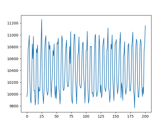
Here is the time series with trend, cycle and random noise. It simulates eCommerce daily sales data with weekly seasonal cycle, linear trend and random Gaussian noise. The sales data is on a per day basis.

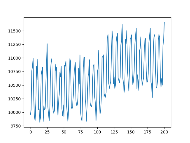
Here is the same time series with anomaly sequence which shifts the mean. It simulates a scenario where the eCommerce sale gets a bump, which could be due to a marketing campaign or a competitor going out of business.

We can clearly see the mean value shifting to higher value. The mean value gradually ramps up and levels off. The driver code for this example is available. A tutorial document for this example is also available.
Wrapping Up
We have gone though an exercise of of creating synthetic time series data using a Python package zaman. The package is designed for use with minimum coding, using a configuration file


