When data is aggregated from various sources in a dynamic environment where the data format might change without any notice, identifying the semantic type of columns in data is a challenging problem. In this post, the problem semantic type identification of data columns will be framed as a classification problem with manually engineered column features. Also, instead of using normal SoftMax label probabilities, we will be using contrastive learning. The solution is available in my OSS GitHub repo whakapai. It’s also available as a Python package called “torvik”.

Column Semantic Type

Currently, most solutions are based on hard coding, regex, and table lookup. However, it’s difficult to scale this kind of solution, especially in dynamic environments with hundreds if not thousands of column types. Deep Learning, along with manually engineered column features, provides an effective solution.

Our discussion is for the semantic type of data, e.g name, address, etc., and not an atomic data type. Semantic type corresponds to some real-world concept e.g., name, address. There may be many semantic types for the same data type, like string.

Existing approaches fall into one of 3 categories hard coding, regular expression, and dictionary look-up. None of these approaches is robust or scalable. However, some semantic types have a well-defined structure and can be defined with regular expressions e.g. email and phone number. For them, existing approaches will suffice.

Deep Learning Solution

The solution presented here is inspired by the solution presented in this paper. However, instead of using normal SoftMax based classification, I have used contrastive learning

The deep learning based solution consists of the following steps. it requires extensive manual feature engineering of column data. For feature engineering, I have used my Python package matumizi which has about 100 data exploration functions. Many of them can be used for feature extraction

• Calculate columns features
• Train a Deep Learning Network for contrastive learning
• Make prediction for column type

There are many column features. This paper cited above lists close to 100 column features. For our use case, I have used the following features. They are based on statistics of certain features in the column data fields e.g. no of numeric characters.

• Mean and std dev of number of alphabetic characters
• Mean and std dev of number of numeric characters
• Mean and std dev of of lengths of field values
• Mean and std dev of number of blank characters

You have to choose the features for a data column based on your knowledge of the column data. Here are some other examples of features. All these features can also be calculated using the matumizi package.

• Fraction of column values with alphabetic characters
• Mean no of certain character in column values
• Min or max no of certain character in column values
• Whether all column values have a certain character
• Skewness in the distribution of certain character count in column values

The data preparation consists of the following steps. The contrastive learning model uses triplet loss. So the training data needs to be in the triplet format. In triplet format, each record consists of a reference or anchor sample followed by a positive sample and a negative sample. For the first step, you should provide many small files with 50 – 100 rows in each for tabular data. Large files need to be split into files of smaller size

• Extract features from the column data. If you have C no of columns and you are extracting F no of features from each column, then will be F number of fields in each record. There will be C no of records from a given file
• Put the data in triplet format i.e. sample record, followed by a positive example and negative example in each record.

The data used for the use case here is customer data. Only 3 column types are being used, i.e. name, address, and city.

In Contrastive Learning during training, the distances in the representation space between a sample and samples of the same class are minimized while the distance with samples of other classes is maximized. Conceptually, it’s like clustering. Contrastive learning has been very useful for vision problems.

The network used is a feed-forward network with only one layer with RELU activation and dropout. The reference sample, positive sample and negative sample are passed through the network, and then triplet loss is applied.

Results

I am using my no-code PyTorch framework called “torvik“, which allows you to train and use a model without any Python coding, with everything defined in a configuration file. Here is the Python implementation for the network. Here is the driver code. Please refer to the tutorial for instructions on how to generate data, train the model and test the model. Here is some sample input. We are using only name, address, and city fields in the data, the data is synthetically generated.

Simona Morasca,3 Mcauley Dr,Ashland,OH,44805,simona@morasca.com
Mitsue Tollner,7 Eads St,Chicago,IL,60632,mitsue_tollner@yahoo.com
Leota Dilliard,7 W Jackson Blvd,San Jose,CA,95111,leota@hotmail.com
Sage Wieser,5 Boston Ave #88,Sioux Falls,SD,57105,sage_wieser@cox.net
Kris Marrier,228 Runamuck Pl #2808,Baltimore,MD,21224,kris@gmail.com

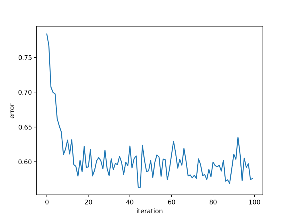
Here is the training error based on triplet loss. PyTorch provides this loss function. But there are other loss functions for contrastive learning.

Here is some test result for one test sample. For each test sample, there are 3 records, because we have three classes of columns Name (N), Address(A), and City(C). Each test record contains the test sample followed of 2 prototype samples of another class. So for each test sample, we will get 3 similarity values. The test sample will be the same class as the prototype samples for which the similarity value is maximum

tensor([0.5533, 0.0000, 0.8760, 0.8455, 0.9100, 0.0000])
tensor([0.5376, 0.0000, 0.8958, 0.8407, 0.9541, 0.0000])
tensor([0.5268, 0.0000, 0.8056, 0.7362, 0.8079, 0.0000])
similarity  1.000  1.000
tensor([0.5533, 0.0000, 0.8760, 0.8455, 0.9100, 0.0000])
tensor([0.4168, 0.0000, 0.0000, 0.0000, 0.1167, 0.5240])
tensor([0.4728, 0.0000, 0.0000, 0.0000, 0.1182, 0.5607])
similarity  0.306  0.307
tensor([0.5533, 0.0000, 0.8760, 0.8455, 0.9100, 0.0000])
tensor([0., 0., 0., 0., 0., 0.])
tensor([0., 0., 0., 0., 0., 0.])
similarity  0.000  0.000

In this case, since the similarity is maximum with the first prototype sample out of 3 for the 3 different classes, the test sample will have have the same class as the first prototype sample. Please refer to the tutorial for the steps to run this use case.

if during prediction time, all similarity scores are below some threshold, then it is some column new semantic type. This will require the model to be retrained with additional training data for the new column type.

Wrapping Up

In this post, we have seen how a Deep Learning model can be used to classify column semantic types in tabular data. Traditional methods for this problem fall short.