What is the relationship between machine learning and optimization? — On the one hand, mathematical optimization is used in machine learning during model training, when we are trying to minimize the cost of errors between our model and our data points. On the other hand, what happens when machine learning is used to solve optimization problems?
Consider this: a UPS driver with 25 packages has 15 trillion possible routes to choose from. And if each driver drives just one more mile each day than necessary, the company would be losing $30 million a year.
While UPS would have all the data for their trucks and routes, there is no way they can run 15 trillion computations per each driver with 25 packages. However, this traveling salesman problem can be approached with something called the “genetic algorithm.” The issue here is that this algorithm requires having some inputs, say the travel time between each pair of locations, and UPS wouldn’t have this information, since there are more than even trillions of combinations of addresses. But what if we use the predictive power of machine learning to power up the genetic algorithm?
The Idea
In simple terms, we can use the power of machine learning to forecast travel times between each two locations and use the genetic algorithm to find the best travel itinerary for our delivery truck.
The very first problem we run into is that no commercial company would share their data with strangers. So how can we proceed with such a project — whose goal would be to help a service like UPS — without having the data? What data set could we possibly use that would be a good proxy for our delivery trucks? Well, what about taxis?—Just like delivery trucks, they are motor vehicles, and they deliver… people. Thankfully, taxi data sets are public because they are provided city governments.
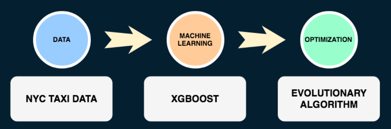
The following diagram illustrates the design of the project: we start with taxi data, use this data to make predictions for travel times between locations, and then run the genetic algorithm to optimize the total travel time. We can also read the chart backwards: in order to optimize the travel time, we need to know how long it takes to get from one point to another for each pair of points, and to get that information, we use predictive modeling based on the taxi data.
Data And Feature Engineering
For illustration purposes, let’s stick to this Kaggle data set, which is a sample of the full taxi data set provided by the city of New York. Data sets on Kaggle are generally well processed and do not always require much work (which is a downside if you want to practice data cleansing), but it is always important to look at the data to check for errors and think about feature selection.
Since we are given each location’s coordinates, let’s calculate the Manhattan distances between each pair of points and count the longitude and latitude differences to get a sense of direction (East to West, North to South). We can clean up timestamps a little and keep the original features which might look useless to us at first glance.
When working with geospatial data, Tableau is a very useful alternative to mapping data points in pandas. A quick preliminary check on the map shows that some drop off locations are in Canada, in the Pacific Ocean, or on the Ellis Island (Statue of Liberty), where cars simply don’t go. Removing these points is quite a difficult task without built-in geo-oriented packages, but we can also leave them in the data, since some machine learning models can deal very well with outliers.

As a bonus, Kaggle conveniently provides data for New York City weather in 2016. This is something we might want to look into in our analysis. But because there are many similar weather conditions—partly cloudy or mostly cloudy—let’s bucket them into major ones to have a smaller variation for these specific features. We can do it in pandas like this:
sample_df["Conditions"] = sample_df["Conditions"].fillna('Unknown')

weather_dict = {'Overcast' : 0,
                'Haze' : 0,
                'Partly Cloudy' : 0,
                'Mostly Cloudy' : 0,
                'Scattered Clouds' : 0,
                'Light Freezing Fog' : 0,

                'Unknown' : 1,
                'Clear' : 2,

                'Heavy Rain' : 3,
                'Rain' : 3,
                'Light Freezing Rain' : 3,
                'Light Rain' : 3,

                'Heavy Snow' : 4,
                'Light Snow' : 4,
                'Snow' : 4}
sample_df["Conditions"] = sample_df["Conditions"].apply(lambda x: weather_dict[x])
Picking The Right Model
With our data and goals, a simple linear regression won’t do. Not only do we want to have a low variance model, we also know that the coordinates, while being numbers, do not carry numeric value for the given target variable. Additionally, we want to add direction of the route as a positive or negative numeric value and try supplementing the model with the weather data set, which is almost entirely categorical.
With a few random outliers in a huge data set, possibly extraneous features which came with it, and a number of possible categorical features, we need a tree-based model. Specifically, boosted trees will perform very well on this particular data set and be able to easily capture non-linear relationships, accommodate for complexity, and handle categorical features.
In addition to the standard XGBoost model, we can try the LightGBM model because it is faster and has better encoding for categorical features. Once you encode these features as integers, you can simply specify the columns with categorical variables, and the model will treat the accordingly:
bst = lgb.train(params,
                dtrain,
                num_boost_round = nrounds,
                valid_sets = [dtrain, dval],
                valid_names = ['train', 'valid'],
                categorical_feature = [20, 24]
                )
These models are fairly easy to set up, but are much harder to fine-tune and interpret. Kaggle conveniently offers root mean squared logarithmic error (RMSLE) as the evaluation metric, since it reduces error magnitude. With RMSLE, we can run different parameters for tree depth and learning rate and compare the results. Let’s also create a validation “watchlist” set to track the errors as the model iterates:
dtrain = xgb.DMatrix(X_train, np.log(y_train+1))
dval = xgb.DMatrix(X_val, np.log(y_val+1))

watchlist = [(dval, 'eval'), (dtrain, 'train')]
gbm = xgb.train(params, dtrain, num_boost_round = nrounds, evals = watchlist, verbose_eval = True )
Optimization With Genetic Algorithm
Now, the machine learning part is only the first step of the project. Once the model is trained and saved, we can start on the genetic algorithm. For those who don’t know, in the genetic algorithm a population of candidate solutions to an optimization problem is evolved toward better solutions, and each candidate solution has a set of properties which can be mutated and altered. Basically, we start with a random solution to the problem and try to “evolve” the solution based on some fitness metric. The result is not guaranteed to be the best solution possible, but it should be close enough.

Let’s say we have 11 points on the map. We would like our delivery truck to visit all these locations on the same day, and we want to know the best route. However, we don’t know how long it will take the driver to go between each point because we don’t have the data for all address combinations.
This is where the machine learning part comes in. With our predictive model, we can find out how long it will take for a truck to get from one point to another, and we can make predictions for each pair of points.
When we use our model as a part of the genetic algorithm, what we start with is a random visit order for each point. Then, based on the fitness score being the shortest total time traveled, the algorithm attempts to find a better visit order, getting predictions from the machine learning model. This process repeats until we figure out a close to ideal solution.
Results
After testing both predictive models, I was surprised to find out that the more basic XGBoost with no weather data performed slightly better than LightGBM, giving a mean absolute error of 4.8 minutes against LightGBM’s 4.9 minutes.
After picking XGBoost and saving the model, I passed it to my genetic algorithm to generate a sample solution and make a demo. Here is a visualization of the end result: we start at a given location, and the genetic algorithm together with machine learning can plan out the optimal route for out delivery truck.

Note that there is a little loop between points 3–4–5–6. If you look closely at the map, you will see that the suggested route goes through the freeway, which is a faster and shorter drive than the residential area. Also, note that this demo is not the exact route planner—it merely suggest the visit order.
Next Steps
Route planning would be the next logical step for this project. For instance, it is possible to incorporate Google Maps API and plan out the exact pathing between each pair of points. Also, the genetic algorithm assumes static time of the day. Accounting for time of the day, while important, is a much more complex problem to solve, and it might require a different approach to constructing the input space altogether.
If you have any questions, thoughts, or suggestions, please feel free to reach out to me on LinkedIn. Code and project description can be found on GitHub.
Thanks for reading!
Source: Travel Time Optimization With Machine Learning And Genetic Algorithm
Transforming Enterprises with
Data & AI Services & Solutions.
ThirdEye delivers Data and AI services & solutions for enterprises worldwide by
leveraging state-of-the-art Data & AI technologies.